
"Which test did you use here?" — a supervisor's question, asked months into data collection, unsettles more graduate students than any statistical table ever printed, because the answer never starts inside SPSS. It starts with the research question itself. Students who open the software first and then hunt for a test that "fits" usually end up with a result that does not answer their question, or a test whose assumptions their data cannot support — followed by a request to redo the chapter. This guide puts the sequence back in order: the three questions that determine the test family before you touch a keyboard, the normality check that settles half the decision, a complete selection table covering the seven tests most used in theses and dissertations, worked APA-style result sentences for each, a fully worked example from hypothesis to final paragraph, and the errors reviewers spot first.
The rule that precedes any test: three determinants
Choosing a statistical test is not a matter of taste, nor of "stronger is better". It is the mechanical application of three questions you can answer from your own data sheet:
First: what is the question looking for? There are exactly three families. Differences (does the mean differ between groups?), associations (do two variables move together?), and prediction (can one variable be estimated from others?). "Does anxiety differ between men and women?" is a difference question. "Are daily phone hours related to anxiety scores?" is an association. "Can anxiety be predicted from phone hours and age together?" calls for regression.
Second: what types of variables are involved? A continuous quantitative variable (a score out of 100, age in years, income), a categorical variable (gender, major, city), and an ordinal variable (satisfaction: low/medium/high). Confusing ordinal with continuous is the single most common source of wrong test choices: a single Likert item is generally ordinal, while the summed score of a full validated scale — reliability checked via Cronbach's alpha as covered in our reliability guide — can usually be treated as continuous.
Third: are the groups independent or paired? Two different samples of people are independent groups; before-and-after measurements on the same people are paired. Running an independent-samples test on pre-post data wastes statistical power and tells a supervisor the basics are shaky.
Once the three answers are on paper, the required test is pinned to one row of the selection table below. This data-first logic is the same foundation as our step-by-step SPSS questionnaire analysis walkthrough — that guide executes inside the software; this one settles the decision that comes before it.
Step zero: is your data normally distributed?
Before any parametric test (t-tests, ANOVA, Pearson, regression), one assumption decides the battle: do your data follow the normal distribution? This is not academic decoration. Parametric tests compute means and standard deviations, and those summaries lose their meaning under heavy skew or extreme outliers. Diagnosis comes from three mutually reinforcing sources:
| Tool | When to use | What you read |
|---|---|---|
| Shapiro-Wilk test | Small to medium samples (rule of thumb: up to ~50) | p below .05 means the data are not normally distributed |
| Kolmogorov-Smirnov test | Larger samples (with Lilliefors correction in SPSS) | Same reading; better suited to big datasets |
| Histogram and Q-Q plot | Always, alongside the test | Bell shape visually; points falling on the straight line |
The practical rule after diagnosis: normal distributions (plus acceptable variance homogeneity via Levene's test) earn you the stronger parametric test; otherwise you move to its non-parametric counterpart that requires no normality — the pairs are listed in full in the table.
One nuance widely missed: in large samples the normality tests turn "significant" on trivial departures that do not matter in practice. So combine all three sources rather than reading one p-value alone; an obvious skew statistic alongside a healthy plot in a sample of 400 argues the overall shape is acceptable despite the test's verdict. SPSS adds a quick numeric assist in the descriptive table: skewness and kurtosis values, with the working rule that staying within ±1 (some references tolerate ±2 in large samples) is an additional acceptance indicator worth citing in your methods chapter next to Shapiro-Wilk or K-S results.
Read the Q-Q plot with simple logic: the points are your ordered values plotted against the values expected under normality. Points tracking the straight line mean acceptable normality; an S-bend means a flat-topped distribution; a curve pulling away at one end means skew and probable outliers at that end. Ten seconds of visual inspection can settle an argument a single test statistic would have prolonged.
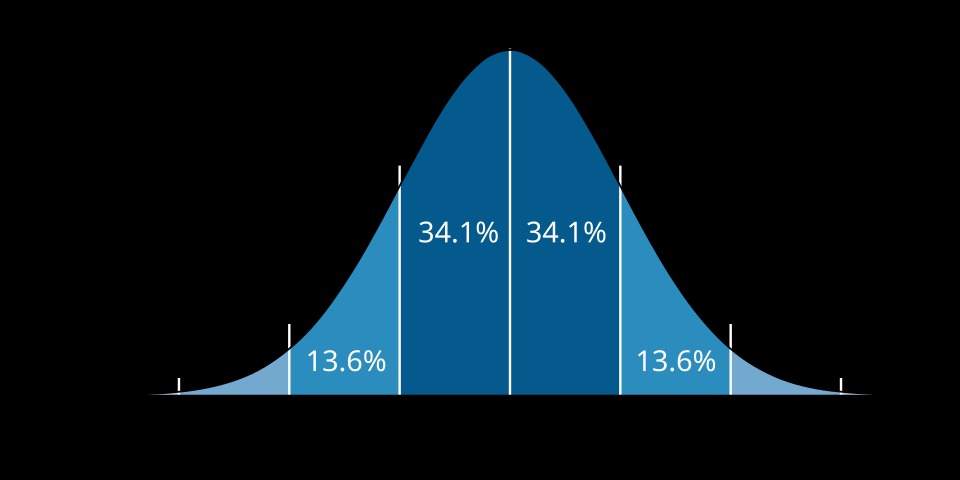
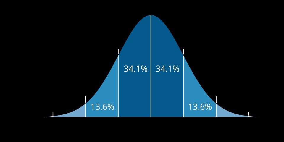
The normal distribution curve with the share of area within each standard deviation of the mean (image: Wikimedia Commons, CC BY 2.5) — many tests assume your data trace something close to this bell
The statistical test selection table
The table gathers the seven tests that dominate theses across fields, read left to right: what is being compared, the assumption, the parametric test when the assumption holds, and its non-parametric alternative when it does not:
| What you compare | Assumption | Parametric test | Non-parametric alternative |
|---|---|---|---|
| Means of 2 independent groups (men/women) | Normality within each group | Independent-samples t-test | Mann-Whitney U |
| 2 paired measurements (pre/post, same people) | Normality of the differences | Paired-samples t-test | Wilcoxon signed-rank |
| Means of 3+ groups (three universities) | Normality + homogeneity of variance | One-way ANOVA | Kruskal-Wallis |
| Association between 2 continuous variables | Normality + linear relationship | Pearson correlation | Spearman correlation (ordinal or skewed) |
| Association between 2 categorical variables | Expected counts ≥ 5 | Chi-square (non-parametric by nature) | — |
| Predicting a continuous variable from one predictor | Linearity + normal residuals | Simple linear regression | — |
| Predicting a continuous variable from several predictors | Linearity + no severe multicollinearity | Multiple regression | — |
How to use the table in your thesis: identify the row from your research question (difference between two independent groups? row one), check the assumption column using the normality section above, and the test name that remains is what you run and what your hypotheses attach to. State in your methodology that assumptions were verified before running — one such sentence raises chapter quality in reviewers' eyes more than a page of theory padding.
Two notes on the table. Chi-square is inherently non-parametric because it works with counts, not means, so it needs no alternative. And when your design measures the same people repeatedly across three or more time points, the design calls for repeated-measures ANOVA, which carries its own assumptions about missing data sphericity.
A significant ANOVA still leaves the question "which groups differ?" unanswered — that is what post-hoc comparisons (Tukey, Bonferroni) are for, and reporting ANOVA without locating the difference is an incomplete result in the eyes of most committees.
Writing results in APA style for the results chapter
Running the test is half the journey; the other half is writing its result in the format journals and committees recognize — APA style. A well-formed sentence carries three layers: descriptive statistics (means and standard deviations), the inferential result (test statistic and p-value), and an effect size saying the difference is large, not merely present.
Copy-ready templates with hypothetical numbers for every test in the table:
Independent-samples t-test: "Anxiety scores were higher among women (M = 42.6, SD = 9.1) than men (M = 38.4, SD = 8.7), a statistically significant difference, t(198) = 2.41, p = .019, d = 0.63."
Paired-samples t-test: "Stress declined after the training programme (M = 21.3, SD = 5.2) relative to baseline (M = 27.8, SD = 6.0), t(49) = 6.15, p < .001, d = 0.87."
One-way ANOVA: "University membership had a significant effect on academic achievement, F(2, 147) = 5.13, p = .007, η² = .15; Tukey post-hoc comparisons located the difference between universities A and C (MD = 6.9, p = .004) with no other pair differing."
Chi-square: "Major was significantly associated with intention to drop out, χ²(2, N = 300) = 11.42, p = .003; the proportion of hesitant students in the humanities track (32%) was double that of the science track (16%)."
Pearson correlation: "Sleep hours were moderately and negatively correlated with anxiety, r(198) = -.44, p < .001." Non-significant results get the same structure with no hedging: "Years of experience showed no significant correlation with job satisfaction, r(148) = .09, p = .256" — a null result is a scientific finding, not an inconvenience to delete.
Spearman correlation: "Job rank was positively associated with satisfaction, rs = .38, p < .001."
Mann-Whitney U: "Men outperformed women on the test, U = 1204.5, Z = -2.71, p = .007, with a medium effect size (r = .27)."
The APA formatting rules that hold it together: no leading zero on p-values (.019, not 0.019); anything below .001 is written exactly as p < .001; statistics letters are italicized in the final text (M, SD, t, F, p); decimals go to two places generally and three for p; the sample size appears inside the parentheses because the reader needs it to judge the inference.
This is precisely where most theses break: raw SPSS output in English is pasted wholesale into the results chapter, or translated so loosely the meaning dissolves. The screenshot below is what the software hands you — the craft lies in converting tables like it into the APA sentences above with the correct effect size for each test.
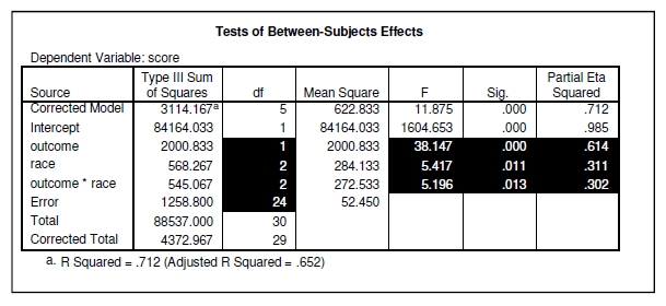
Raw ANOVA output in SPSS (image: Wikimedia Commons, public domain — IBM); the templates above are what these numbers must become in your results chapter
A complete worked example: from hypothesis to final paragraph
To assemble the whole picture: a researcher studies "the effect of a presentation-skills programme on public-speaking confidence" with 60 students in two groups — experimental and control — using a 100-point confidence scale administered before and after the programme.
Hypotheses. "There is no significant difference between the experimental and control groups on post-programme confidence scores" is the null, against an alternative of a significant difference. Note the hypothesis names one variable, one scale, one measurement point — not the vague "the programme improves confidence".
Data screening. Completion 100%, no missing values, no out-of-range scores (high 88, low 22). Normality of difference scores: Shapiro-Wilk p = .310 (experimental) and p = .240 (control); histograms acceptable; Levene's test p = .520. Documented decision: assumptions hold, the parametric route is open.
Test selection. Two independent groups with pre and post measurements. The most precise choice is ANCOVA using the pre-score as covariate, but a widely accepted practical equivalent compares the difference scores between groups with an independent-samples t-test — the route taken here for illustration.
Reading the output. Mean difference score: experimental 14.2 (SD = 5.1), control 1.3 (SD = 4.8). The t table returns t(58) = 9.87, p < .001, Cohen's d = 2.55; degrees of freedom equal both samples minus two.
The final APA paragraph, as it would appear in the results chapter: "To examine the programme's effect on speaking confidence, difference scores (post minus pre) were compared between groups using an independent-samples t-test, after verifying normality and homogeneity of variance assumptions. Results showed a significant difference favouring the experimental group (M = 14.2, SD = 5.1) over the control group (M = 1.3, SD = 4.8), t(58) = 9.87, p < .001, d = 2.55, a large practical effect."
What the sequence buys you: every number in the final paragraph traces to a prior step — the hypothesis selected the test, the assumption check justified the parametric choice, the output converted to a standard sentence, and the effect size closes the door on "statistically significant, but does it matter?" Repeat the chain for every hypothesis in the thesis; five hypotheses produce five such paragraphs, each shorter than this example because the study context is stated once at the top of the chapter.
Common errors that ruin the decision before it starts
Running many tests "to be sure". Some students run t, Mann-Whitney, and Kruskal-Wallis on the same comparison, then report whichever came out significant. Reviewers recognize the pattern, and it weakens every result that follows. Choose once, by the logic here, and report once.
Ignoring outliers. One mis-keyed value (age 999) can flip a distribution and the test with it. Check ranges and extremes first; then correct documented entry errors or remove with stated, defensible reasons.
Confusing significance with importance. Large samples produce significance from trivial differences. Always report the effect size — as the templates do — and discuss practical importance, never p alone.
Difference tests on association questions. "Are grades related to income?" is a correlation question, yet it is sometimes forced into a t-test by splitting income into high/low groups. Splitting discards information; correlation or regression answers directly.
Rushing the instrument. The entire structure stands on a reliably coded instrument; a questionnaire that never passed design and reliability review — from electronic questionnaire design through reliability testing — undermines every test downstream, because the software analyses the codes, not the meanings behind them.
Treating a null result as proof of absence. "The study proved there are no differences" is an inference error. Failing to reject the null means your sample found insufficient evidence of a difference — possibly because of sample size. Write "the results showed no significant difference", report means and the effect size, and note a possible power limitation; committees read that candour as competence.
Under-auditing demographic tables. Descriptive tables come first in most theses and are the easiest for a committee to check; percentages that do not total 100 or counts exceeding the sample size open doubt over everything after them. Give them the same scrutiny as the hypothesis tests.
From selection to the finished chapter
The final working sequence: derive hypotheses from the research question, screen the data (completeness, outliers, normality, Levene), select the test from the table, run it and read the output, write it in APA form, then interpret it theoretically in the discussion chapter — linking numbers to prior studies, not repeating them. Before submitting any results chapter, run it against this list: every hypothesis has a matching result and vice versa; every test is named with a one-sentence methodological justification; every result carries descriptives, test statistic, exact p, and effect size with italics applied; no screenshots of software appear in the chapter body (rebuilt tables in the body, raw output in an appendix if required); non-significant results are present and fully written; and no theoretical interpretation appears inside the results chapter — interpretation lives in the discussion.
Doctoral applicants in particular need this chain complete, because funded PhD programmes in Europe and Asia — such as the currently open funded doctoral positions — increasingly expect a credible analysis plan in the proposal, and research tools like Perplexity AI Pro for academics help with the literature side but cannot make this methodological decision for you.
If you have reached this line with half-clean data and a deadline closing in, the SPSS statistical analysis service from Truescho runs the whole chain — assumption checking, test selection matched to your questions, APA-formatted writing of results, and an explanation of every step so you can defend it in your viva — under an explicit policy of never fabricating or altering data.
Want someone to handle the analysis for you? The Truescho team runs the statistical tests and writes your results in APA form — request the service now.
Frequently asked questions
How do I choose the right statistical test for my research?
Answer three questions before opening any software: is your question about a difference, an association, or a prediction? Are your variables continuous, categorical, or ordinal? Are the groups independent or paired? The three answers pin the test to one row of the selection table; then check the normality assumption if the candidate test is parametric, and switch to its non-parametric counterpart if it fails.
What is the difference between a t-test and ANOVA?
A t-test compares the means of exactly two groups, while one-way ANOVA compares three or more groups in a single procedure, protecting you from the inflated Type I error that comes from running multiple pairwise t-tests on the same groups. A significant ANOVA still needs post-hoc comparisons, such as Tukey, to locate which pairs differ.
When should I use Mann-Whitney instead of a t-test?
Use Mann-Whitney U when comparing two independent groups whose data fail the normality assumption, or when your dependent variable is ordinal to begin with. It compares ranks instead of means, so skew and outliers do not distort it — it is the direct non-parametric counterpart of the independent-samples t-test.
Should I use Pearson or Spearman correlation?
Pearson fits two continuous variables when both are roughly normal and the relationship is linear; Spearman fits ordinal data, visibly skewed distributions, or monotonic but non-linear relationships. As a working rule, check normality and the scatterplot first — and when in doubt, Spearman loses little and protects much.
How do I report test results in APA style?
The standard sentence combines descriptives first, then the statistic with degrees of freedom and p-value, then the effect size — for example, t(198) = 2.41, p = .019, d = 0.63. Symbols are italicized, p carries no leading zero and three decimals, and anything below .001 is reported simply as p < .001.
Where is the normality test in SPSS?
Under Analyze, then Descriptive Statistics, then Explore; request "Normality plots with tests" in the Plots settings. The Tests of Normality table then reports Shapiro-Wilk (suitable for smaller samples) and Kolmogorov-Smirnov (for larger ones); a significance value below .05 rejects the normality assumption.
What if my data are not normally distributed?
Three routes exist: switch to the non-parametric alternative from the table (the most common choice in theses), transform the data (logarithmic or square-root) and re-check, or rely on the large-sample justification where the central limit theorem supports robust parametric testing — the last usually needing supervisor approval and a written rationale in the methodology.
Do I need post-hoc tests after ANOVA?
Yes, when the ANOVA is significant. It answers only "is there a difference somewhere among the groups"; post-hoc procedures such as Tukey or Bonferroni identify which pairs actually differ, and reporting a significant ANOVA without locating the difference is treated as an incomplete result by most committees.